Transformer 20-Step Visual Study Notes

This note is based on the interactive explanation from Transformer Explainer. It follows the site’s 20 steps and organizes them into a study note for understanding how GPT-style Transformers perform next-token prediction. The site uses GPT-2 small as the example model and visualizes the full pipeline from input tokens to output probabilities.

First, remember one sentence: the core task of GPT-style Transformers is next-token prediction. Given the prompt:

Data visualization empowers users to

The model needs to answer:

What is the most likely next token?

To answer this, a Transformer goes through tokenization, embedding, positional encoding, repeated Transformer blocks, self-attention, MLP, logits, probability distribution, sampling strategy, and other steps.

All screenshots in this note are taken from Transformer Explainer, developed by the Georgia Tech Polo Club team. They are used here for personal study notes. It is best to read this together with the original interactive site.

What Is Transformer

Transformer is the most common foundation architecture for modern large language models. Text-generation models such as GPT, Llama, and Gemini can all be understood as expanded versions of the Transformer architecture.

Its most important ability is not “memorizing answers”, but learning language patterns from large amounts of text and then predicting the next token from context at inference time. This prediction is repeated: predict one token, append it to the text, then predict the next one.

Step 1: What is Transformer

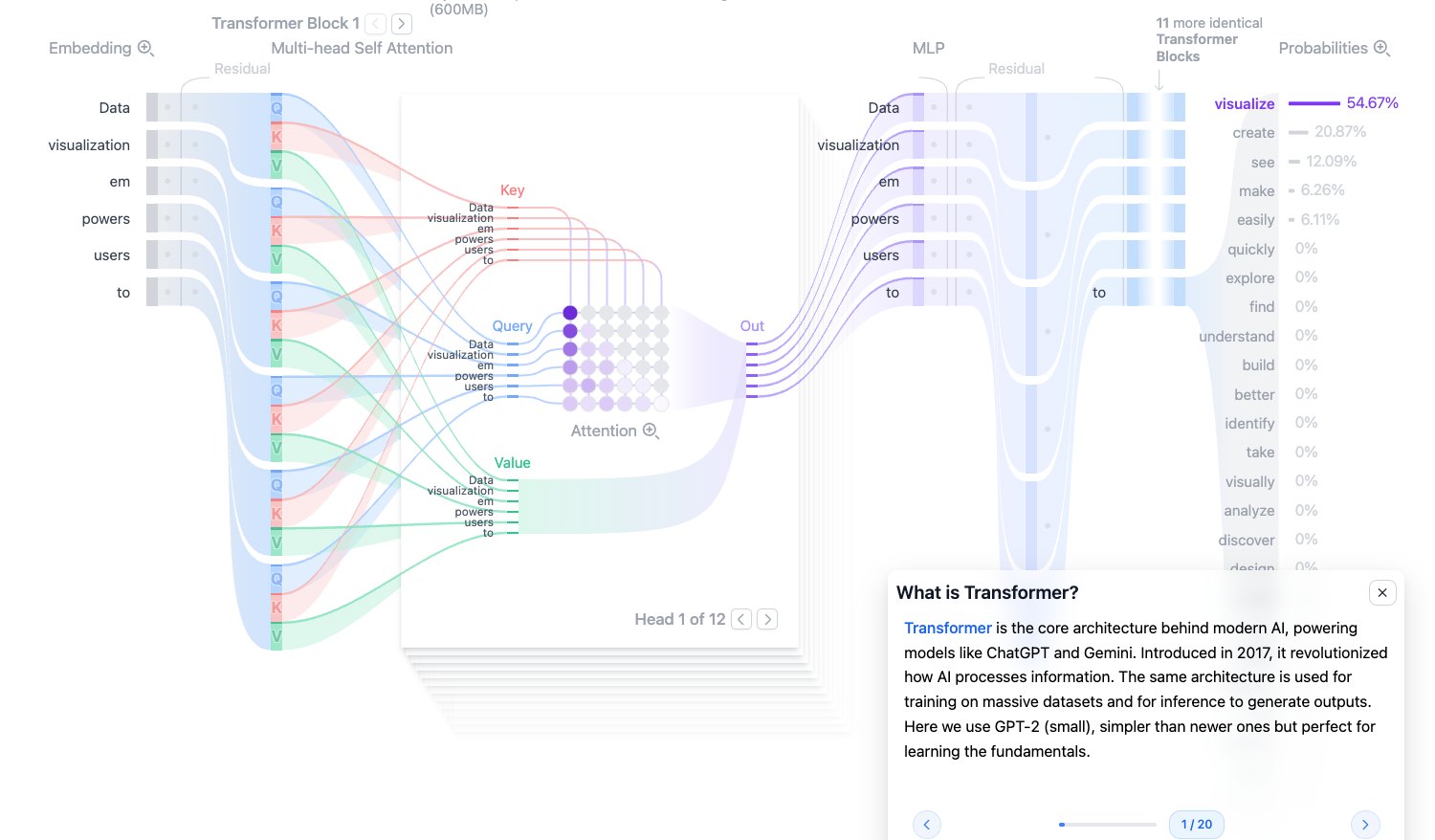
Source: Transformer Explainer, https://poloclub.github.io/transformer-explainer/

How Transformers Work

When a Transformer generates text, it does not write an entire paragraph at once. It generates step by step. Each step performs the same task: predict a probability distribution for the next token based on the existing context.

For example, if the current input is:

Data visualization empowers users to

The model may assign the highest probability to visualize, while also assigning relatively high probabilities to tokens such as create, see, and make. The final selected token is also affected by sampling parameters such as temperature, top-k, and top-p.

Step 2: How Transformers Work

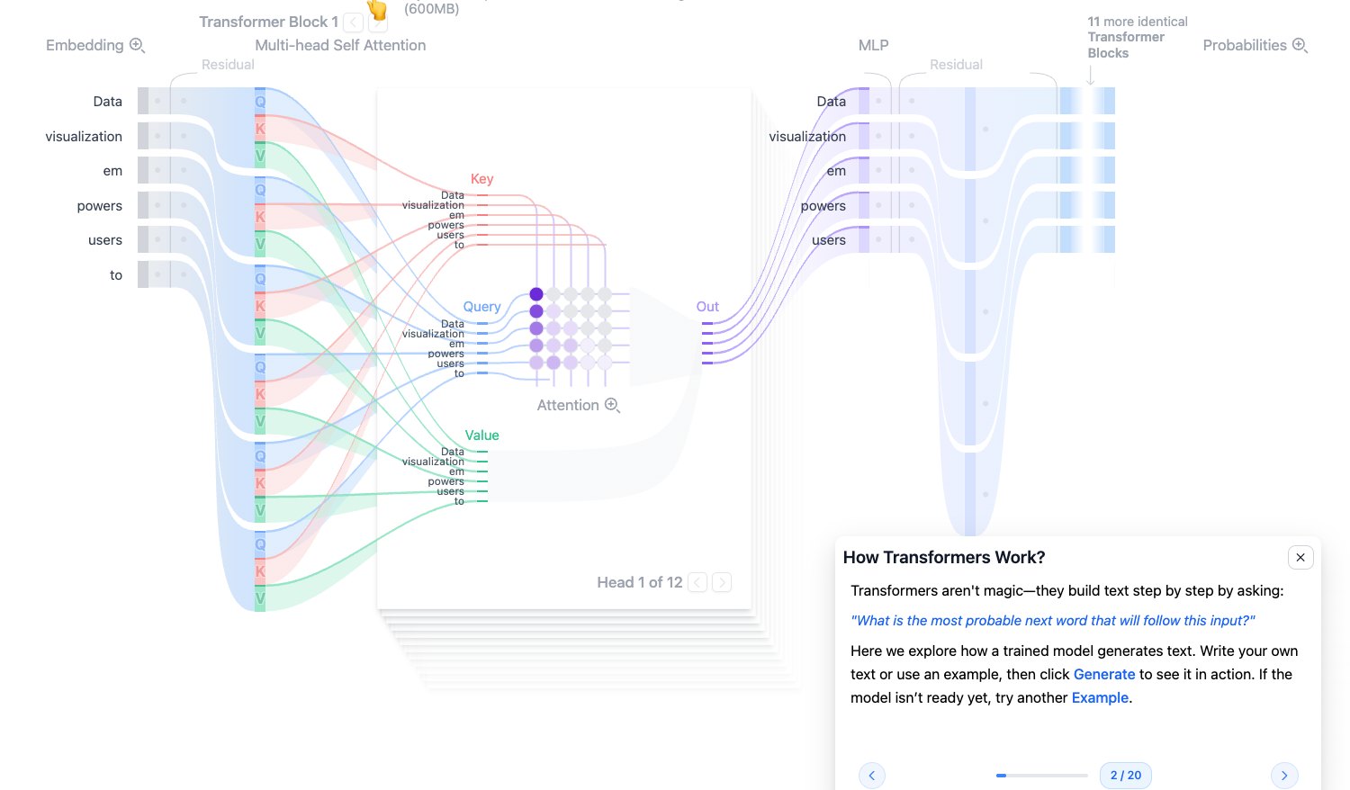
Source: Transformer Explainer

Transformer Architecture

A text-generation Transformer can be divided into three major parts:

Embedding: converts human-readable text into vectors the model can process.
Transformer Blocks: repeatedly refine each token representation, mainly through Self-Attention and MLP.
Output Probabilities: converts the final vector into probabilities over all tokens in the vocabulary.

At a high level, the information flow is:

text input -> token -> embedding -> Transformer Blocks -> logits -> probabilities -> sample next token

Step 3: Transformer Architecture

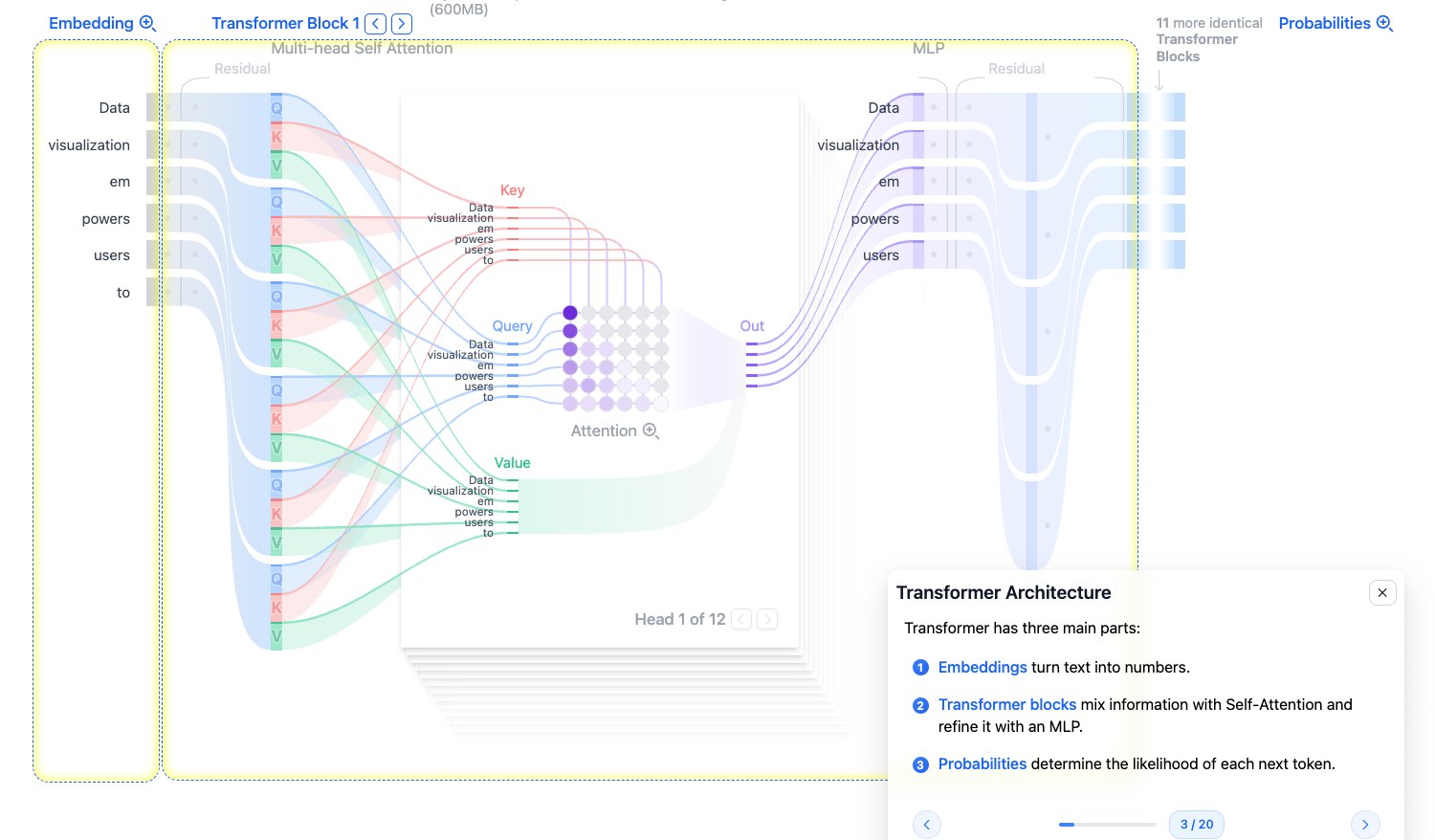
Source: Transformer Explainer

Embedding

The model cannot directly understand strings. Embedding converts each token into a sequence of numbers, or a vector. This vector is not manually designed; it is learned during training.

If two tokens often appear in similar contexts, their embeddings tend to be closer in high-dimensional space. You can think of embedding as an internal “semantic coordinate” used by the model.

GPT-2 small has a hidden dimension of 768, so each token is represented as a 768-dimensional vector.

Step 4: Embedding

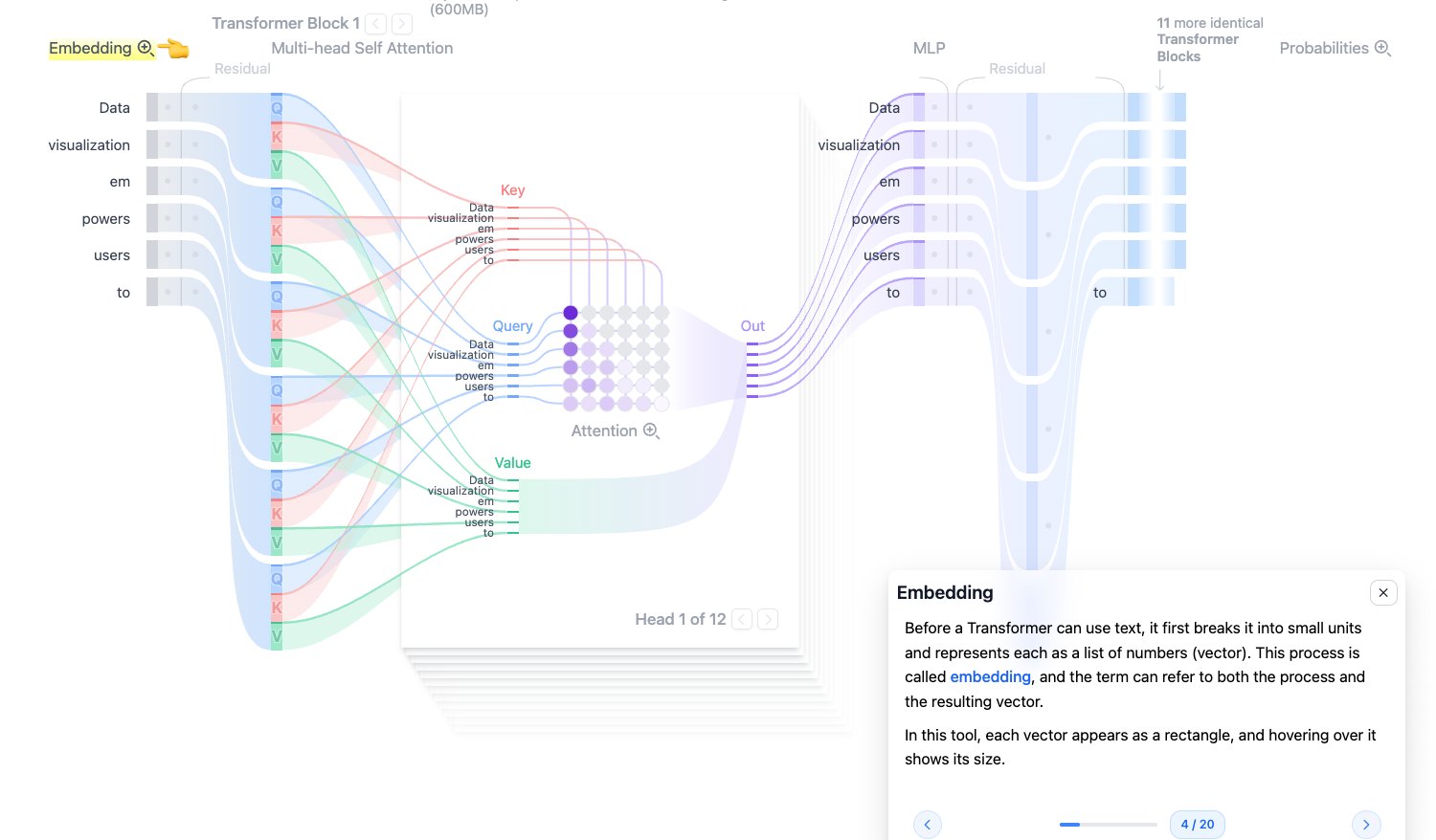
Source: Transformer Explainer

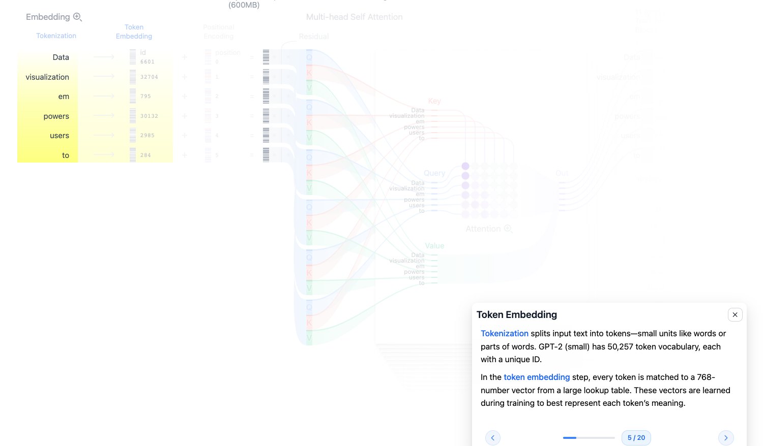
Token Embedding

Tokenization splits input text into tokens. A token can be a full word or a subword. For example, empowers in the example is split into em and powers.

Each token has a unique ID. GPT-2 has a vocabulary size of 50,257, so its token embedding matrix is roughly:

$$ 50257 \times 768 $$

After the model gets the token ID, it looks up the corresponding 768-dimensional vector from this large matrix.

Step 5: Token Embedding

Source: Transformer Explainer

Positional Encoding

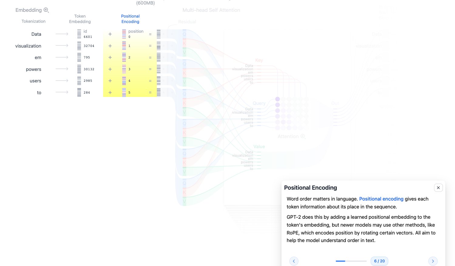
Self-Attention does not naturally know sequence order. If the model only receives a set of token vectors, it does not know which token comes first and which comes later.

So positional encoding is needed. GPT-2 uses learnable positional embeddings and adds the semantic token vector and the position vector:

$$ x_i = \text{TokenEmbedding}_i + \text{PositionEmbedding}_i $$

This lets the model know both “what this token is” and “where it is.”

Step 6: Positional Encoding

Source: Transformer Explainer

Repetitive Transformer Blocks

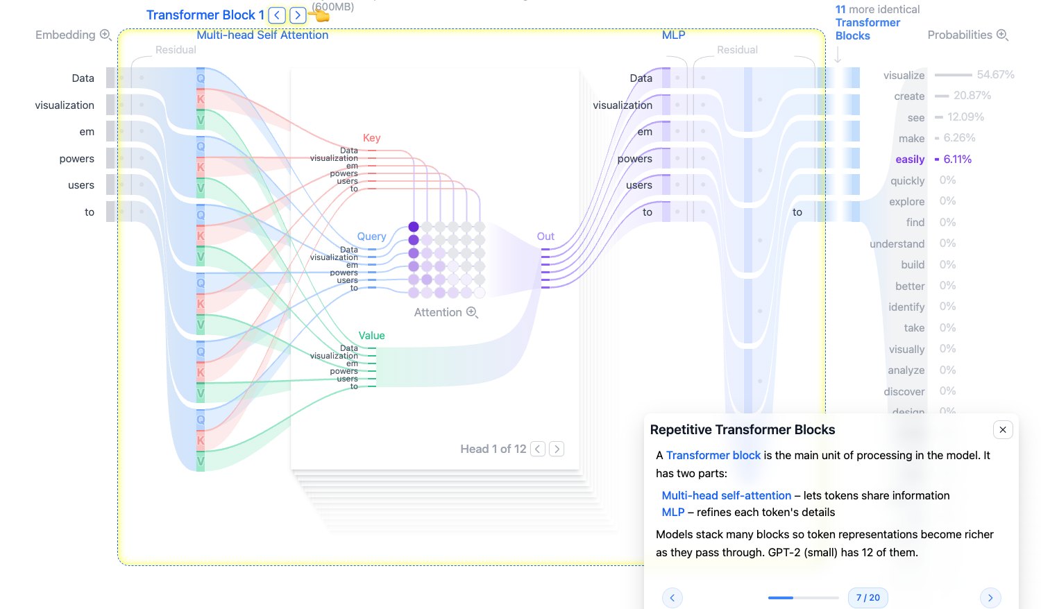
Embedding is only the input representation, not a fully contextualized semantic representation. The real context modeling happens inside Transformer Blocks.

GPT-2 small has 12 Transformer Blocks. Each block roughly contains:

Multi-Head Self-Attention: lets tokens exchange information.
MLP: nonlinearly processes each token representation.
Residual, LayerNorm, and Dropout: stabilize training and improve generalization.

The meaning of stacking multiple layers is that lower layers tend to capture local and lexical information, while higher layers more easily form complex semantic and task-related representations.

Step 7: Repetitive Transformer Blocks

Source: Transformer Explainer

Multi-Head Self Attention

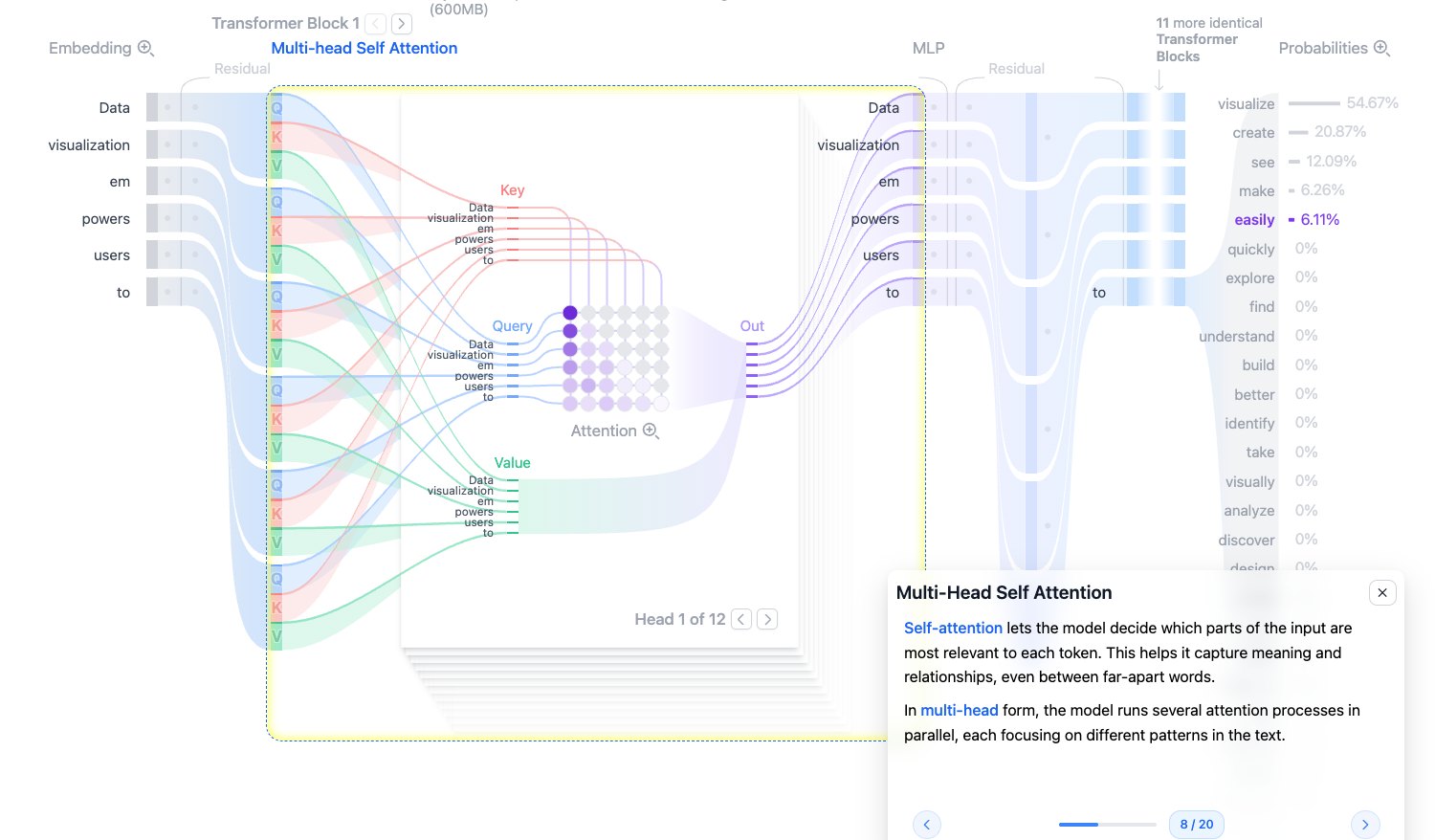
The goal of Self-Attention is to let each token update itself based on context. For example, the token to has different meanings in different sentences. It needs to “look at” the previous context Data visualization empowers users to form a more accurate representation.

Multi-Head means the model does not use just one attention perspective. It uses multiple heads in parallel. GPT-2 small has 12 attention heads. Different heads can learn different relationships, such as syntactic relations, short-distance collocations, and long-distance semantic dependencies.

Step 8: Multi-Head Self Attention

Source: Transformer Explainer

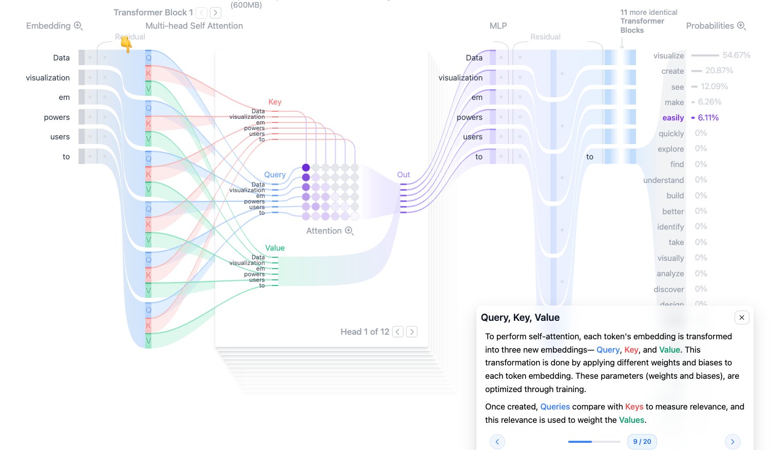
Query, Key, Value

Self-Attention maps each token’s input vector into three vectors:

Query (Q): what information the current token wants to search for.
Key (K): features by which each token can be matched by others.
Value (V): the actual information content to be aggregated and passed along.

They come from linear transformations:

$$ Q = XW_Q,\quad K = XW_K,\quad V = XW_V $$

A simple analogy is a search engine:

Query is the search query.
Key is the page title or index.
Value is the page content.

The model first computes relevance between Query and Key, then reads Value with weighted aggregation.

Step 9: Query, Key, Value

Source: Transformer Explainer

Multi-Head

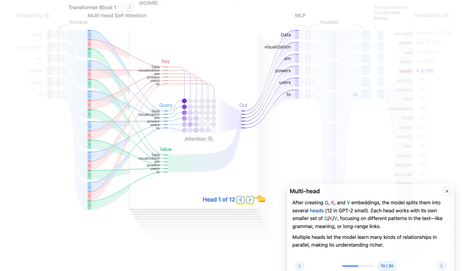
GPT-2 small has an embedding dimension of 768 and 12 attention heads, so each head usually processes:

$$ 768 / 12 = 64 $$

The benefit of multi-head attention is learning multiple relationships in parallel. One head may focus on adjacent words, another on subject-verb relationships, and another on more distant semantic hints.

Multiple heads are not duplicate work; they give the model multiple “viewing angles.”

Step 10: Multi-head

Source: Transformer Explainer

Masked Self Attention

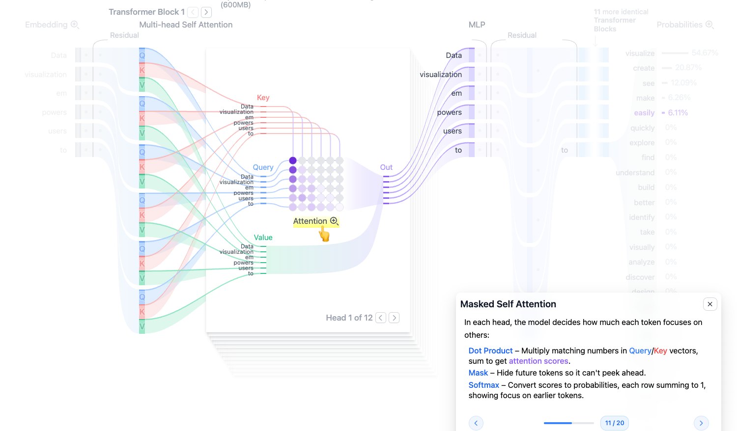
GPT-style models generate text from left to right. When predicting the current position, they must not peek at future tokens, so causal mask, also called masked self-attention, is used.

The core formula is:

$$ \text{Attention}(Q,K,V)=\text{softmax}\left(\frac{QK^T}{\sqrt{d_k}} + M\right)V $$

Where:

$QK^T$: computes pairwise similarity between tokens.
$\sqrt{d_k}$: scaling factor that prevents dot products from becoming too large and making softmax too sharp.
$M$: mask matrix that sets future positions to $-\infty$.
softmax: turns scores into probabilities.
multiplying by $V$: aggregates information according to attention weights.

Step 11: Masked Self Attention

Source: Transformer Explainer

Attention Output and Concatenation

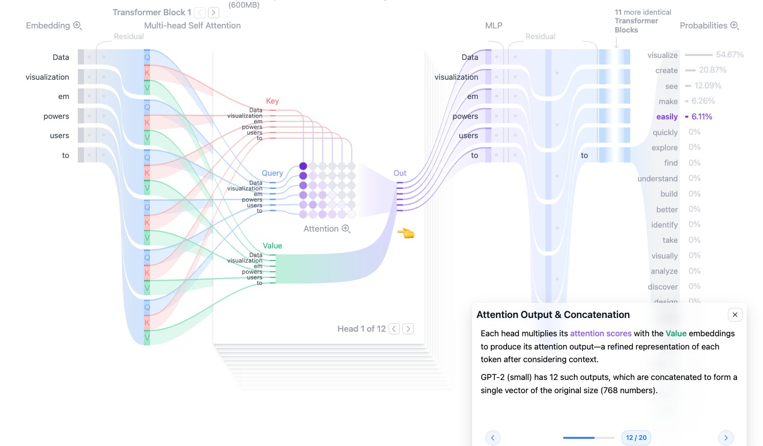
Each head outputs a context-enhanced token representation. Since GPT-2 small has 12 heads, it produces 12 sets of results.

The model then concatenates the outputs from these heads and applies a linear projection back to the original hidden dimension 768:

head_1, head_2, ..., head_12 -> concat -> linear projection

The purpose is to let different heads extract information separately, then fuse those perspectives into one unified representation.

Step 12: Attention Output & Concatenation

Source: Transformer Explainer

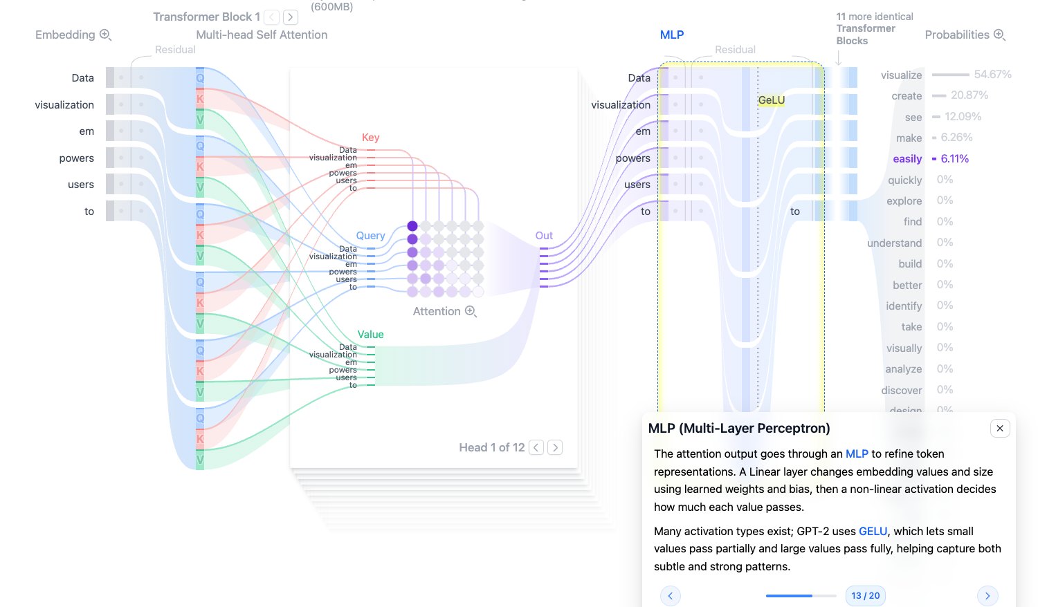
MLP

Attention handles information flow between tokens. MLP processes each token’s own representation nonlinearly.

GPT-2’s MLP usually contains two linear transformations with GELU activation in between:

$$ \text{MLP}(x)=W_2\cdot \text{GELU}(W_1x+b_1)+b_2 $$

The first layer expands the dimension from 768 to 3072, and the second layer compresses it back to 768. Expanding the dimension lets the model represent more complex features in a higher-dimensional space.

Note that MLP does not communicate across tokens like Attention. It processes each token independently.

Step 13: MLP

Source: Transformer Explainer

Output Logit

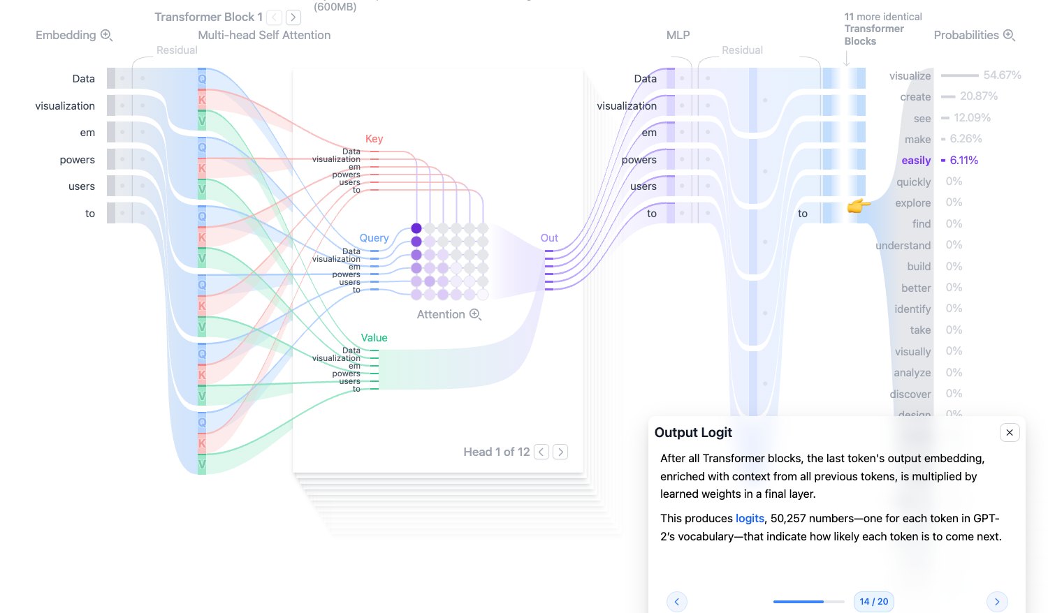
After all Transformer Blocks, the model takes the output vector at the last position and uses it to predict the next token.

This vector goes through the final linear layer and is mapped to the vocabulary size:

$$ \text{logits}=h_{\text{last}}W_{\text{vocab}}+b $$

GPT-2 has a vocabulary size of 50,257, so logits are a vector of length 50,257. Each number corresponds to the raw score of a candidate token.

A logit is not a probability. It can be any real number and must go through softmax to become a probability distribution.

Step 14: Output Logit

Source: Transformer Explainer

Probabilities

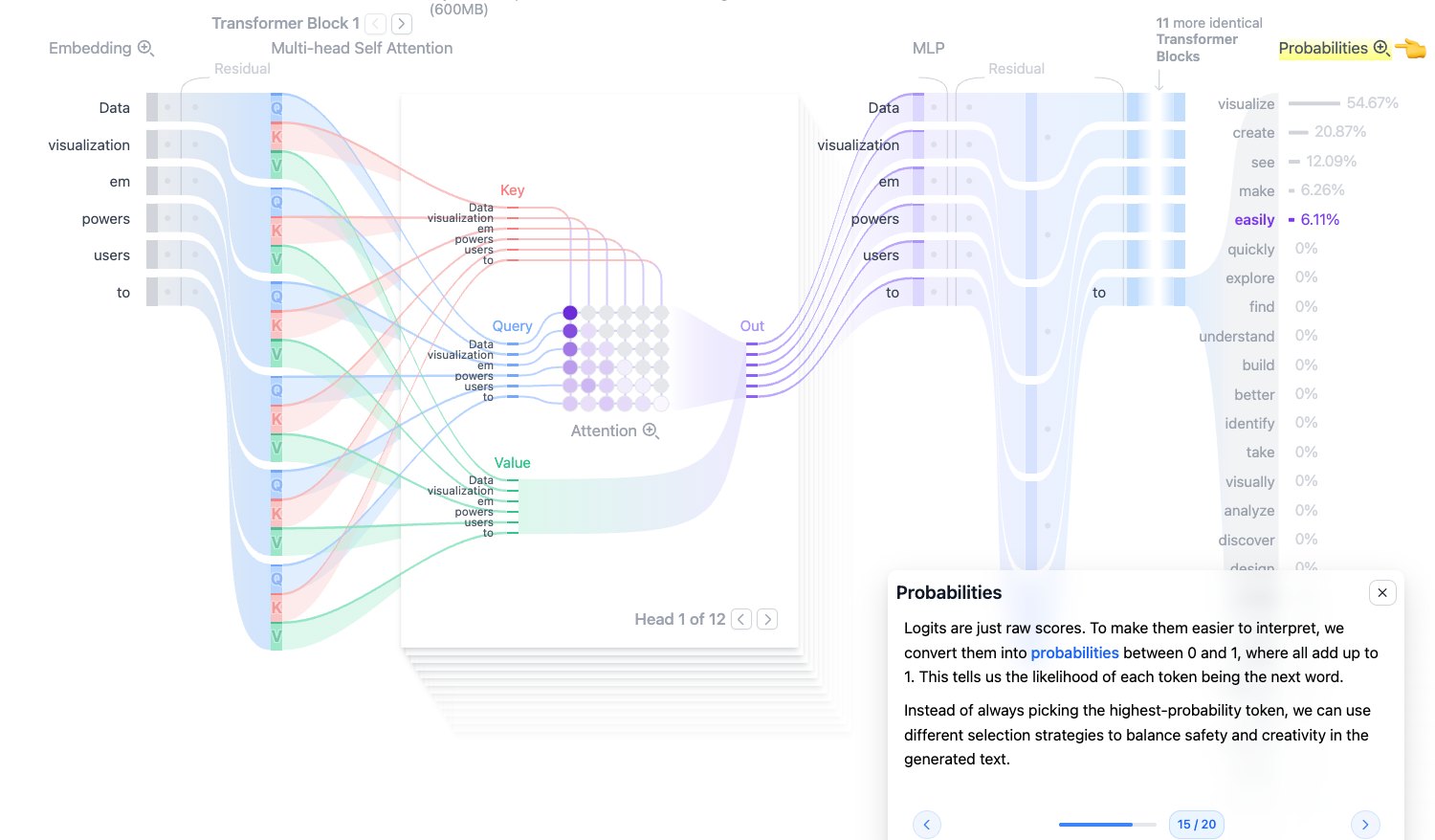
Softmax converts logits into probabilities:

$$ p_i=\frac{e^{z_i}}{\sum_j e^{z_j}} $$

After conversion:

Every token probability is between 0 and 1.
The probabilities of all tokens sum to 1.

In the figure, after the example input, the model considers tokens such as visualize, create, see, and make to be likely next tokens.

Step 15: Probabilities

Source: Transformer Explainer

Temperature

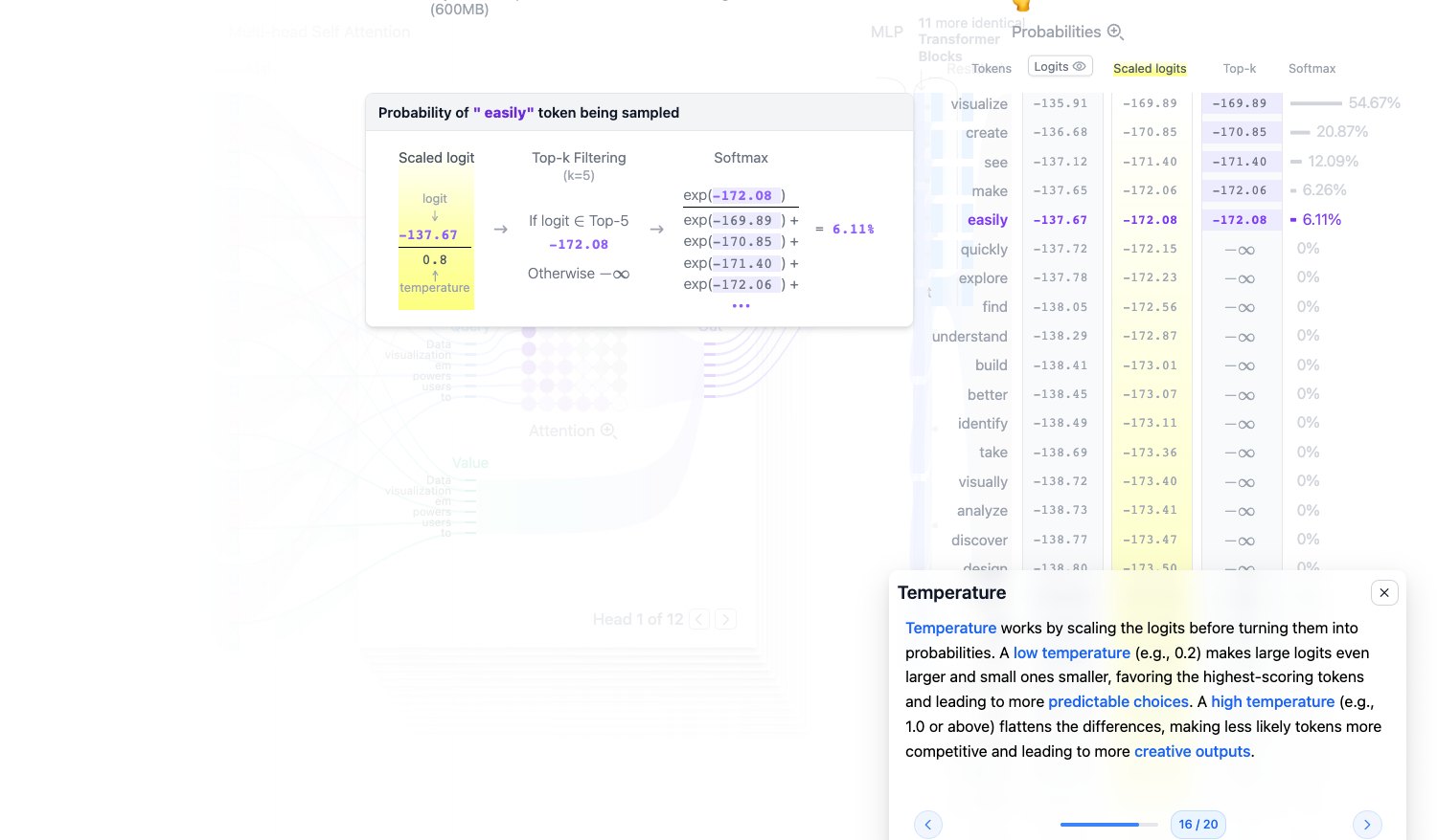
Temperature scales logits before softmax:

$$ p_i=\frac{\exp(z_i/T)}{\sum_j \exp(z_j/T)} $$

Where $T$ is the temperature:

$T < 1$: the probability distribution becomes sharper. High-score tokens are more likely to be selected, and output is more stable.
$T = 1$: logits are not additionally adjusted.
$T > 1$: the probability distribution becomes flatter. Low-probability tokens have more chances to be selected, and output becomes more diverse.

In simple terms, lower temperature is more conservative, while higher temperature is more divergent.

Step 16: Temperature

Source: Transformer Explainer

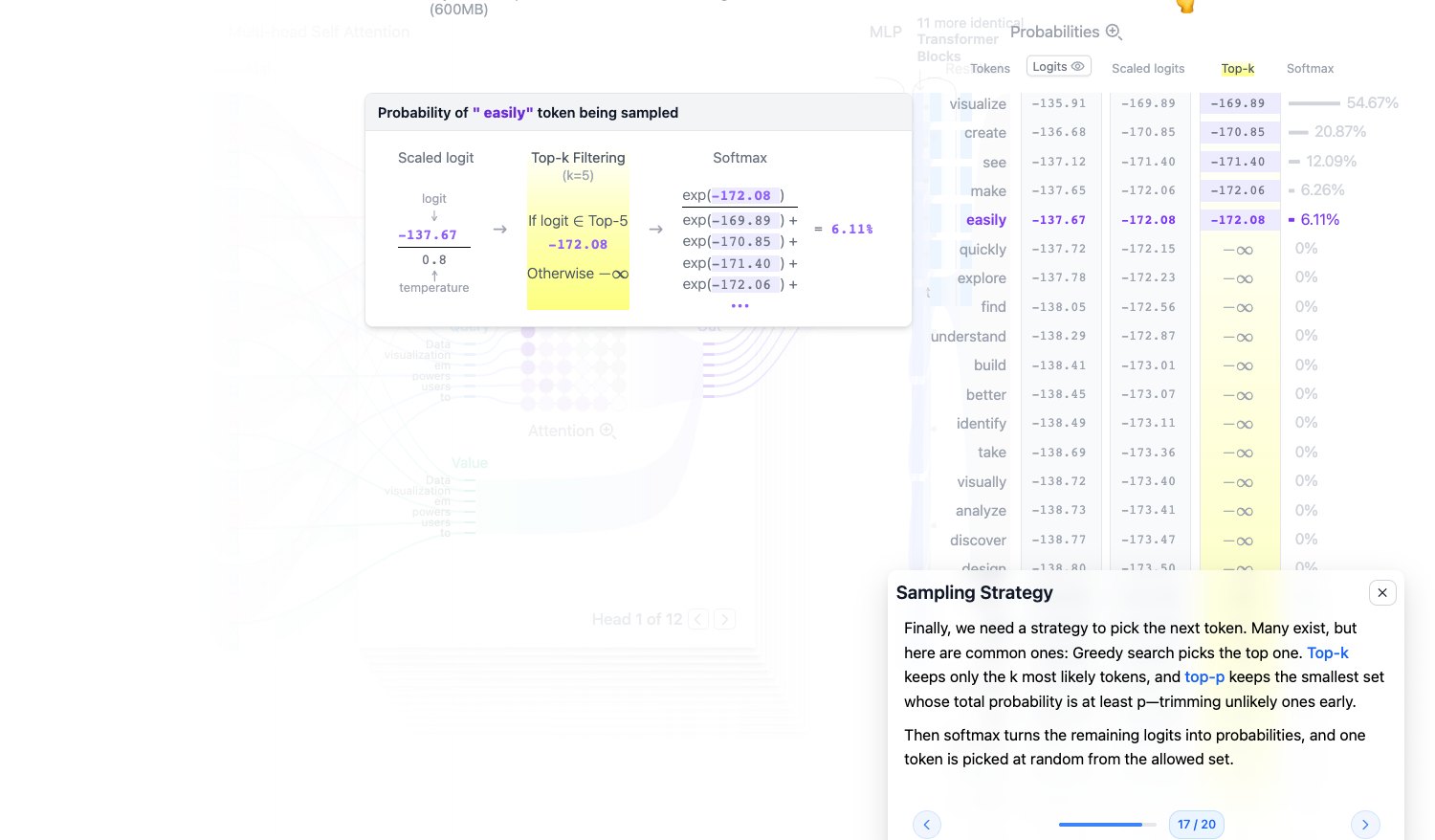
Sampling Strategy

After obtaining a probability distribution, the model still needs to decide how to choose the next token. Common strategies include:

Greedy Search: always choose the highest-probability token. Stable, but can be rigid.
Top-k: keep only the k highest-probability tokens, then sample from them.
Top-p: keep the smallest token set whose cumulative probability reaches p. Also called nucleus sampling.

Top-k is more like a fixed candidate pool, while top-p is a dynamic candidate pool. In practice, temperature and top-k/top-p are often tuned together.

Step 17: Sampling Strategy

Source: Transformer Explainer

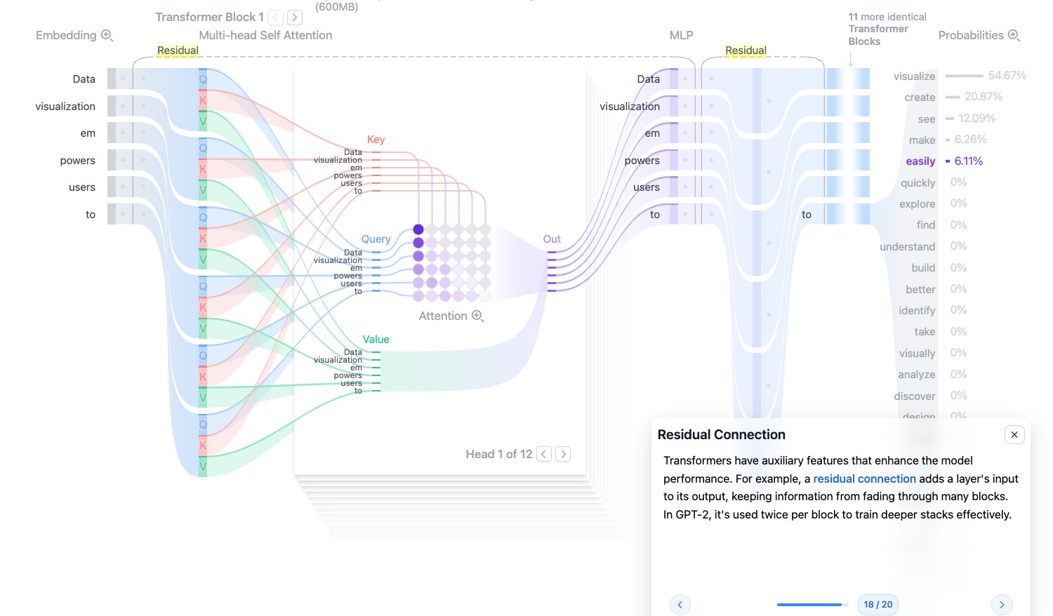
Residual Connection

A residual connection adds a layer’s input directly to its output:

$$ y = x + F(x) $$

Its purpose is to preserve original information and make gradients pass through deep networks more easily. Without residual connections, training becomes harder as the model gets deeper, and information from early layers is more likely to be lost.

In Transformers, residual connections usually surround both Attention and MLP.

Step 18: Residual Connection

Source: Transformer Explainer

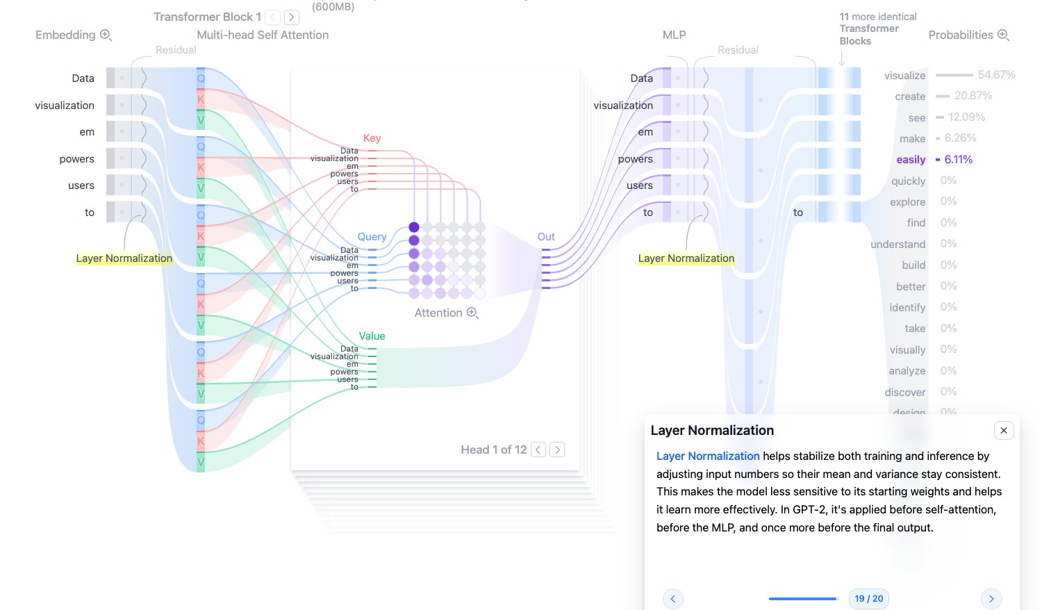
Layer Normalization

Layer Normalization normalizes the values inside a token vector, making the mean and variance more stable:

$$ \text{LayerNorm}(x)=\gamma\frac{x-\mu}{\sqrt{\sigma^2+\epsilon}}+\beta $$

It reduces training instability and makes the input distribution of each layer more controllable. GPT-2 uses a pre-norm style: LayerNorm is applied before entering Attention and MLP.

Intuitively, LayerNorm is like adjusting the numerical scale to a more suitable range before each key computation.

Step 19: Layer Normalization

Source: Transformer Explainer

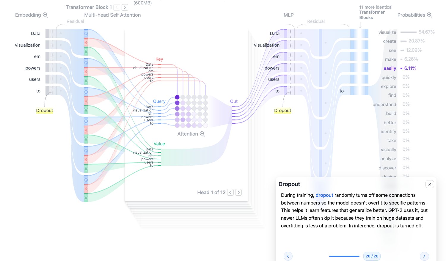
Dropout

Dropout is a regularization method used during training. It randomly sets part of the connections or activations to zero, preventing the model from over-relying on certain local features.

The intuition is: during training, do not let the model follow the exact same path every time, forcing it to learn more robust representations.

Important notes:

Dropout is mainly used during training.
Dropout is disabled during inference.
Many newer large models use less Dropout than early models because their training data is extremely large.

Step 20: Dropout

Source: Transformer Explainer

One Flowchart Summary

The inference flow of a GPT-style Transformer can be compressed into this chain:

flowchart LR
    A["Input text"] --> B["Tokenization"]
    B --> C["Token Embedding"]
    C --> D["Positional Encoding"]
    D --> E["Transformer Block x N"]
    E --> F["Multi-Head Self-Attention"]
    F --> G["MLP"]
    G --> H["Final Linear"]
    H --> I["Logits"]
    I --> J["Softmax Probabilities"]
    J --> K["Temperature / Top-k / Top-p"]
    K --> L["Sample next token"]

Key Differences from RNN

Combining this with the previous RNN note, the difference can be understood like this:

Aspect	RNN	Transformer
Information transfer	Passed step by step through hidden state	Self-Attention lets tokens directly read one another
Parallelism	Strong time-step dependency, hard to parallelize	Tokens in the same layer can be computed in parallel
Long-distance dependency	Long path, easy to decay	Any positions can directly connect
Context representation	Compressed into hidden state	Keeps explicit token representations for the whole context
Large-model training	Less efficient to scale	Better suited to large-scale GPU/TPU matrix computation

This is why modern LLMs mainly use Transformers: they are not only strong in modeling, but also better engineered for large-scale pretraining.