RNN Recurrent Neural Network Study Notes
This note summarizes what I learned from Andrej Karpathy’s classic blog post The Unreasonable Effectiveness of Recurrent Neural Networks. The original article was published in 2015 and uses character-level language models to show how RNNs/LSTMs can learn spelling, formatting, structure, local syntax, and even interpretable “state memory” from raw text.
The main thread of this note is:
- Why RNNs are suitable for sequences.
- The core formulas and computation process of RNNs.
- How character-level language models are trained and sampled.
- What the classic experiments in Karpathy’s article demonstrate.
- Why RNNs were later replaced by Transformers in mainstream NLP.
What Problem RNNs Solve
Ordinary feedforward neural networks usually assume that inputs and outputs are fixed-length vectors, such as taking an image as input and outputting a class label. But many real tasks are naturally sequential:
- Text: a sentence consists of multiple tokens or characters.
- Speech: audio frames are arranged over time.
- Video: frames are arranged over time.
- Translation: one sentence is converted into another sentence in another language.
- Generation: previously generated content affects what comes next.
The key idea of an RNN is: when processing the current input, the model does not only look at the current input; it also maintains a hidden state that compresses past context.
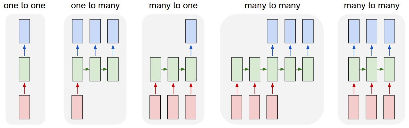
Source: Andrej Karpathy, The Unreasonable Effectiveness of Recurrent Neural Networks. Red represents input, blue represents output, and green represents recurrent state. The diagram shows common modes such as fixed input/output, sequence output, sequence input, sequence-to-sequence, and synchronized sequence input/output.
You can think of an RNN as a repeatedly called step function:
rnn = RNN()
y = rnn.step(x)
Each time step(x) is called, the RNN reads the current input x_t, combines it with the previous hidden state h_{t-1}, updates a new hidden state h_t, and produces the current output y_t.
Core Formula of a Vanilla RNN
The most basic RNN update is:
$$ h_t = \tanh(W_{hh}h_{t-1} + W_{xh}x_t + b_h) $$$$ y_t = W_{hy}h_t + b_y $$Where:
- $x_t$: input at time step $t$
- $h_{t-1}$: hidden state from the previous time step
- $h_t$: hidden state at the current time step
- $W_{xh}$: input-to-hidden weights
- $W_{hh}$: hidden-to-hidden recurrent weights
- $W_{hy}$: hidden-to-output weights
- $\tanh$: nonlinear activation that squashes values into $[-1, 1]$
In code, it roughly looks like this:
class RNN:
    def step(self, x):
        self.h = np.tanh(np.dot(self.W_hh, self.h) + np.dot(self.W_xh, x))
        y = np.dot(self.W_hy, self.h)
        return y
The most important thing to understand is the meaning of h: it is not a hand-written rule, but a “context summary” learned by the model during training. If the input is text, h may carry information such as whether the model is inside quotes, inside a URL, whether a bracket is open, or what words have appeared before.
Why RNNs Can Model Context
Take the string hello as an example. Suppose the vocabulary only contains the four characters h, e, l, o. During training, the input and target can be:
Input:  h e l l
Target: e l l o
Notice that the target after the first l is l, while the target after the second l is o. If the model only looks at the current character, both time steps have the same input, so it cannot tell what the next character should be. The RNN must use its hidden state to record “what has already been seen.”
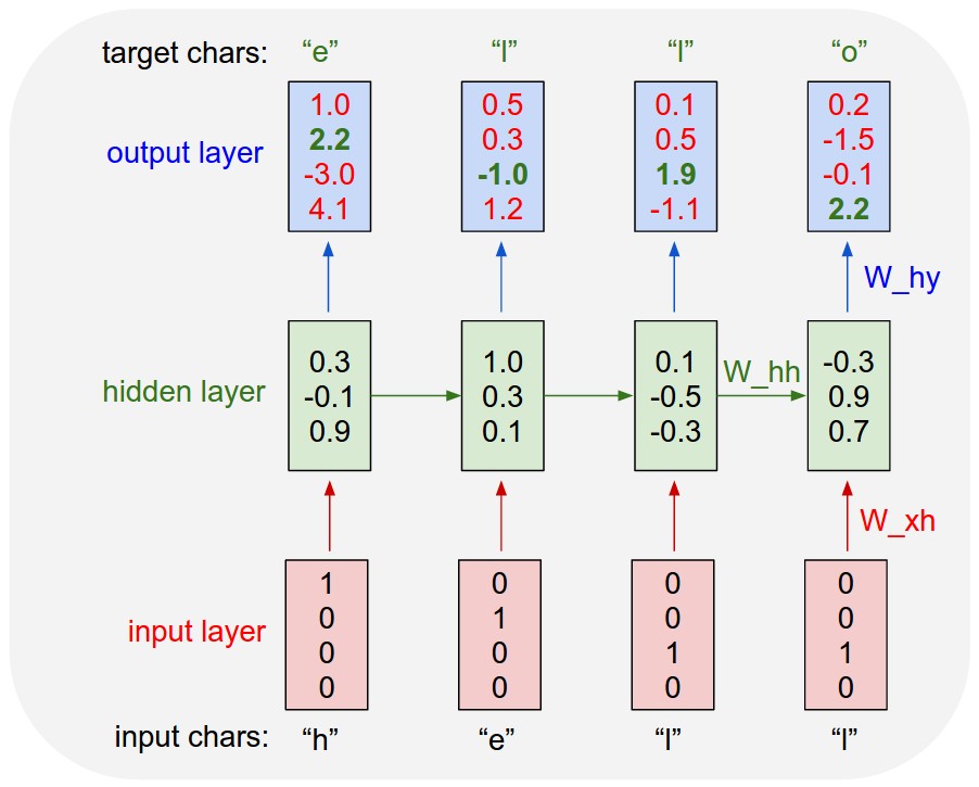
Source: Andrej Karpathy, The Unreasonable Effectiveness of Recurrent Neural Networks. The model reads hell one character at a time, outputs scores for the next character at each step, and the green targets show the correct characters whose scores should be increased.
The training objective is usually cross-entropy loss at every time step:
$$ \mathcal{L} = -\sum_t \log p(x_{t+1}\mid x_{\le t}) $$Where:
- $x_{\le t}$ means the context up to and including the current position.
- $p(x_{t+1}\mid x_{\le t})$ means the probability of the next character predicted from historical context.
After training, text generation works as follows:
- Give the model a starting character or prompt.
- Get the probability distribution for the next character.
- Sample one character from the distribution.
- Feed the sampled character back into the model.
- Repeat the process.
This is the simplest generation loop for a character-level language model.
BPTT: How RNNs Are Trained
An RNN reuses the same set of parameters at every time step. During training, the recurrent structure is unrolled over time and then backpropagation is applied. This is called Backpropagation Through Time, BPTT.
If the sequence is very long, fully unrolling it is expensive. A common approach is Truncated BPTT, where gradients are only propagated back for a fixed number of steps. For example, Karpathy’s Paul Graham experiment used truncated BPTT with a length of 100 characters.
The main difficulty in RNN training comes from long chains of gradients:
$$ \frac{\partial \mathcal{L}}{\partial h_{t-k}} $$This gradient must pass through many matrix multiplications and nonlinear functions. When the chain is long, gradients may:
- Become smaller and smaller: vanishing gradients, making long-term dependencies hard to learn.
- Become larger and larger: exploding gradients, making training unstable.
This is why LSTM and GRU became widely used.
LSTM: A Stronger Recurrent Unit
The experiments in Karpathy’s article actually use LSTM. LSTM is still part of the RNN family, but it uses a more complex hidden-state update with gates, making it easier for the model to keep or forget information.
Typical LSTM components include:
- Forget gate: decides how much old information to keep.
- Input gate: decides how much new information to write.
- Output gate: decides how much current state to expose to the output.
- Cell state: provides a more stable information channel.
Intuitively, a Vanilla RNN mixes the old state and the new input at every step and compresses them again, so long-term information is easily overwritten. LSTM gives the model mechanisms for “writing, keeping, and reading”, making it more suitable for long sequences.
Classic Experiments in Karpathy’s Article
Learning Structure from Characters
The original article shows RNN/LSTM results trained on different kinds of text, including:
- Paul Graham essays
- Shakespeare plays
- Wikipedia Markdown/XML
- Algebraic geometry LaTeX
- Linux source code
- Baby name lists
The common point is that the model is not given an explicit dictionary, grammar rules, Markdown rules, XML tree rules, or C language rules. It is only trained to “predict the next character.” Yet after training, it can generate text that looks like the distribution of the original data.
This shows that: next-character prediction looks simple, but it forces the model to learn multi-level structure.
- Character level: spelling, spaces, punctuation
- Word level: common words, names, variable names
- Syntax level: quotes, brackets, indentation, tag closure
- Style level: Shakespeare-like dialogue, Wikipedia-like entries, source-code comments
Capability Evolution During Training
Karpathy uses War and Peace as an example to show how sampled text changes over training iterations:
- Early stage: almost random characters, but spaces begin to appear.
- Middle stage: short words, periods, quotes, and other local structures appear.
- Later stage: more English-like words, names, and sentence forms appear.
My understanding is that an RNN does not learn “language” all at once. It first learns the most local and frequent patterns, then gradually forms longer-range dependencies.
Hidden Units Learn Interpretable States
One of the most classic parts of the article is the visualization of LSTM hidden unit activations. Some neurons activate inside URLs, some activate inside Markdown link contexts such as [[...]], and others seem to track quoted regions.
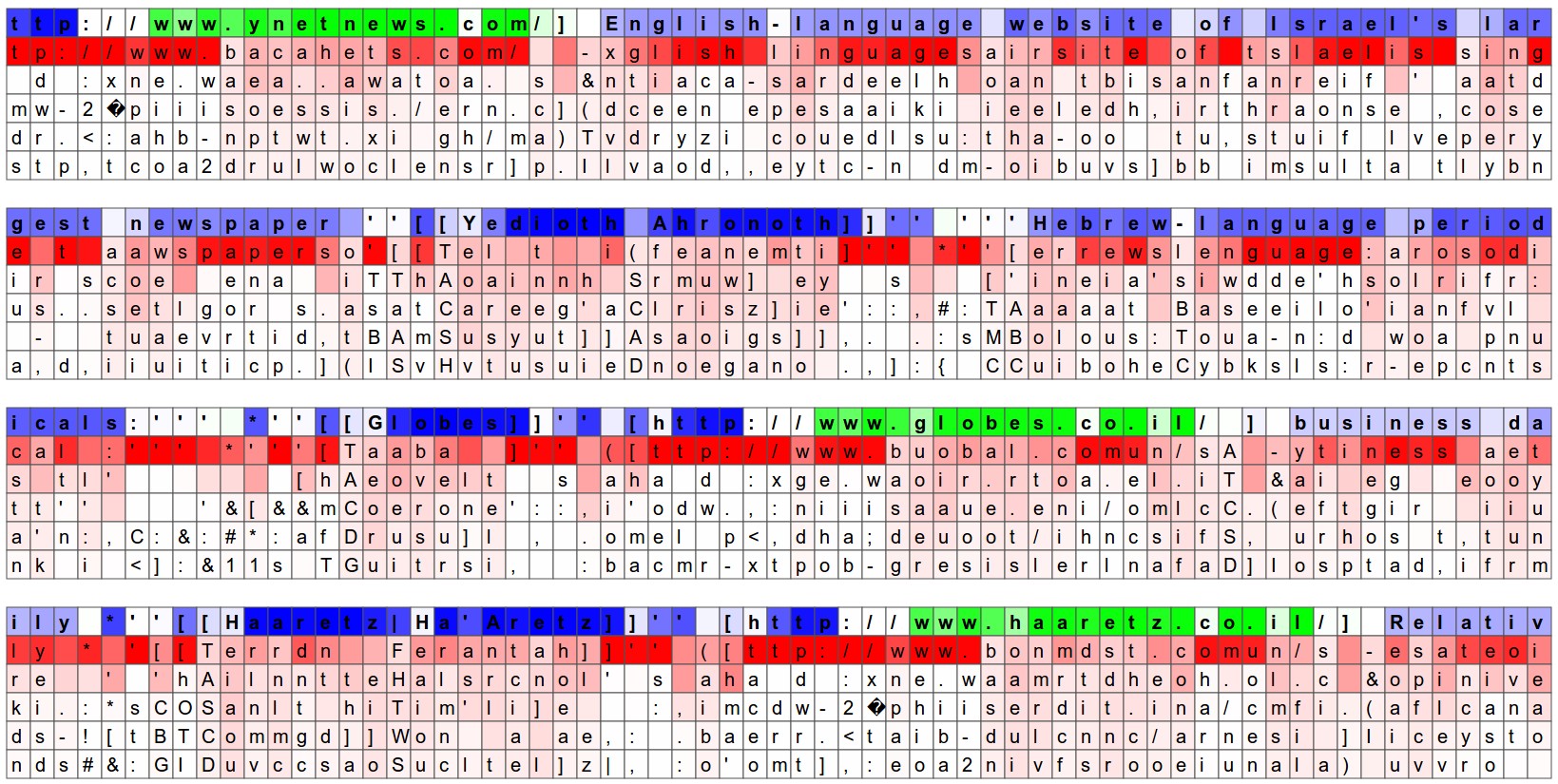
Source: Andrej Karpathy, The Unreasonable Effectiveness of Recurrent Neural Networks. This figure shows a hidden unit that activates strongly in URL regions, suggesting the model may have learned an internal state for “currently inside a URL.”
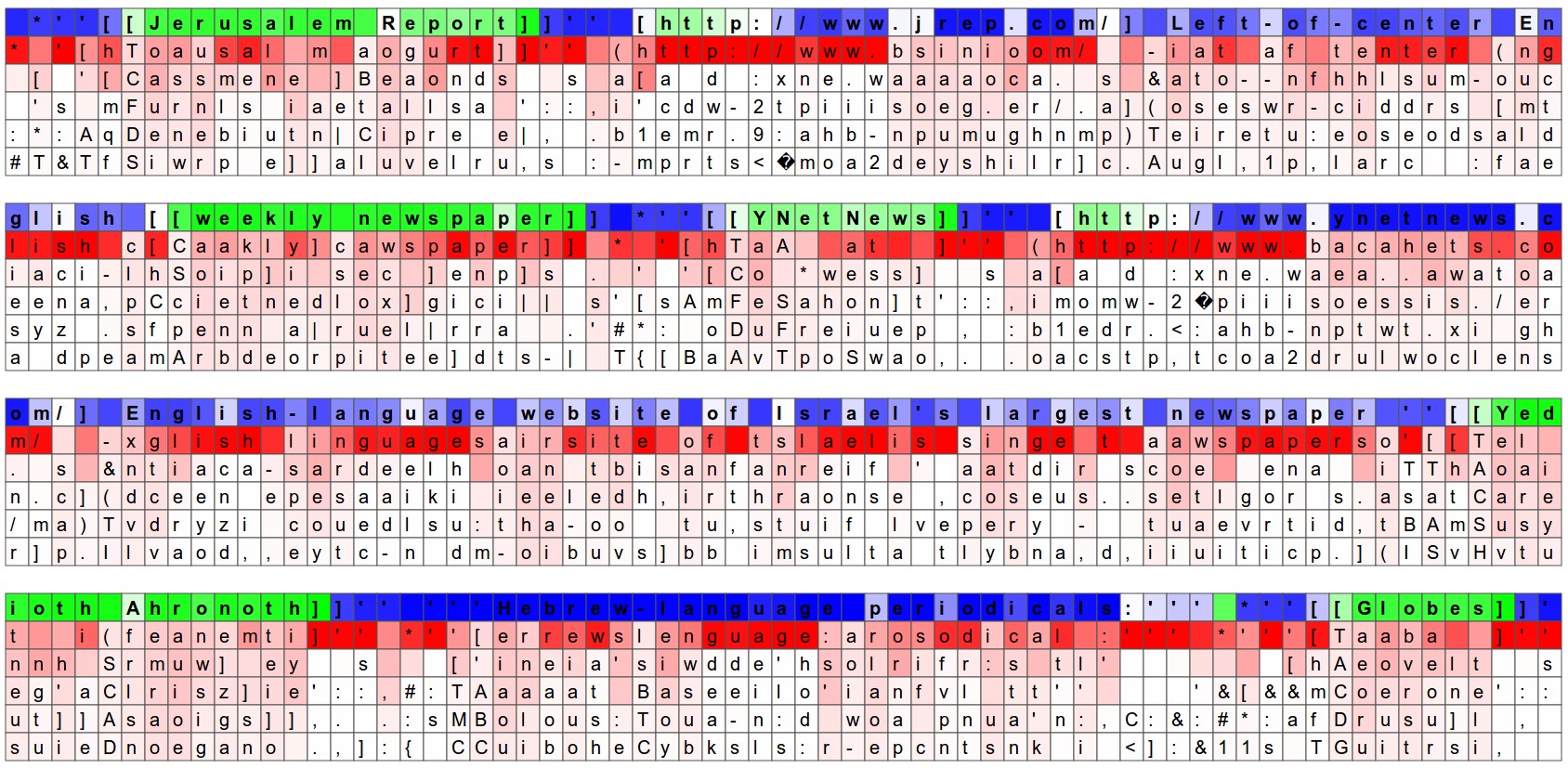
Source: Andrej Karpathy, The Unreasonable Effectiveness of Recurrent Neural Networks. This figure shows a hidden unit responding to the [[...]] Markdown environment.
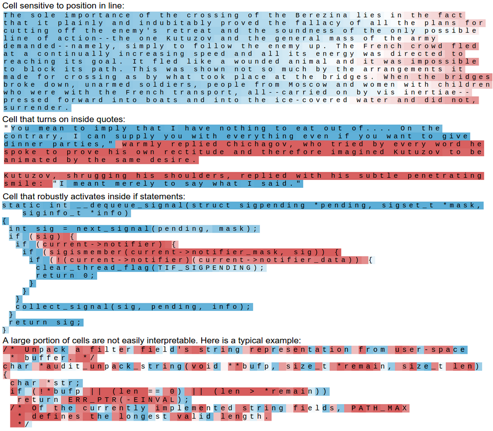
Source: Andrej Karpathy, The Unreasonable Effectiveness of Recurrent Neural Networks. These visualizations show that some hidden units learn state-detection functions that humans can interpret.
The point is not that every neuron has a clear semantic meaning. Rather, end-to-end training can lead the model to discover intermediate states that are useful for the task. For next-character prediction, knowing whether the model is inside a URL, bracket, or quote genuinely improves prediction accuracy.
RNNs Can Handle Non-Traditional Sequential Tasks
Karpathy also mentions that even when the data itself is not a sequence, the processing procedure can be designed as a sequence. For example, a model can move attention step by step to read an image, or generate an image step by step on a canvas.
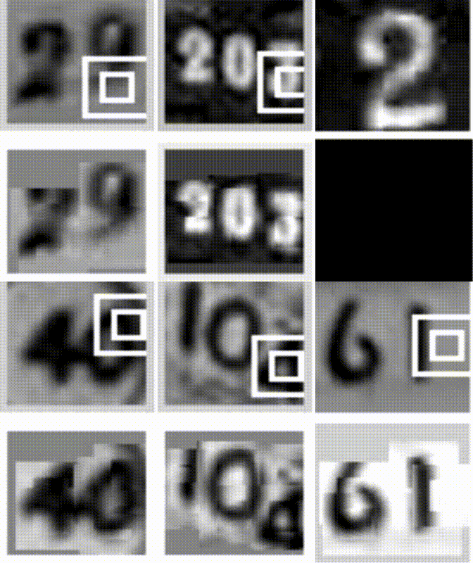
Source: Andrej Karpathy, The Unreasonable Effectiveness of Recurrent Neural Networks. The experiment on the left is related to Recurrent Models of Visual Attention.
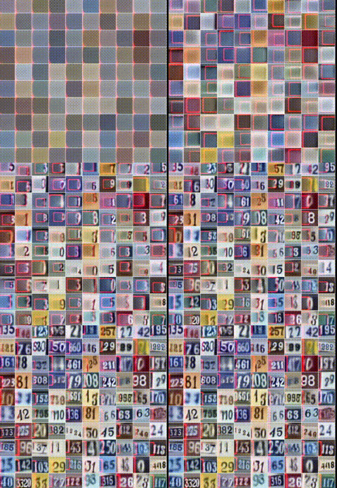
Source: Andrej Karpathy, The Unreasonable Effectiveness of Recurrent Neural Networks. The experiment on the right is related to DRAW: A Recurrent Neural Network For Image Generation.
This gives an important perspective: RNNs are not only for “processing sequence data”; they can also represent “a computation process executed in order.”
Sampling Temperature: Why Generation Changes
A character-level language model outputs a probability distribution for the next character. During sampling, a temperature value is often used to adjust the distribution:
$$ p_i = \frac{\exp(z_i / T)}{\sum_j \exp(z_j / T)} $$Where:
- $z_i$ is the logit of the $i$-th character.
- $T$ is the temperature.
The effect of temperature:
- $T < 1$: the distribution becomes sharper; the model is more conservative and more likely to repeat high-probability patterns.
- $T = 1$: normal sampling.
- $T > 1$: the distribution becomes flatter; output is more diverse, but errors also increase.
So the “creativity” and “stability” of a generative model are often a tradeoff.
Advantages of RNNs
RNN advantages can be summarized as:
- Naturally suitable for streaming input: when data arrives one time step at a time, an RNN can continuously update its state.
- Parameter sharing: the same
stepfunction is reused for sequences of arbitrary length. - State compression: the hidden state can summarize past context.
- Simple generation intuition: predict the next token, then feed the output back into the model.
- Still valuable for small models and certain temporal tasks, such as sensor sequences, real-time speech, and low-latency tasks on edge devices.
Limitations of RNNs
The main limitations are also clear.
Sequential Computation Is Hard to Parallelize
An RNN must compute $h_{t-1}$ before it can compute $h_t$. This means the time steps inside one sequence are hard to fully parallelize.
For short sequences this may not matter much, but in large-scale language model training, both data size and model size are huge. Not being able to fully use GPU/TPU parallelism becomes a core bottleneck.
Long-Distance Dependencies Are Difficult
In theory, the hidden state can carry all historical information. In practice, it is hard for a fixed-length vector to losslessly compress a long context. Earlier information passes through more state updates and is more likely to be overwritten or weakened.
LSTM/GRU mitigate this issue, but do not completely solve it.
The Information Path Is Too Long
If the first token needs to affect the 1000th token, the information in an RNN must pass through about 1000 recurrent updates. The longer the path, the harder optimization becomes and the easier information is lost.
Hidden State Is a Bottleneck
RNNs compress the past into one hidden vector. This vector must both store context and participate in the next computation. Karpathy also mentions in the outlook section that RNNs couple representation capacity with per-step computation cost: the larger the hidden state, the more expensive each matrix multiplication becomes.
Why RNNs Were Replaced by Transformers
Transformers did not replace RNNs because “RNNs are completely useless.” They replaced them because, for large-scale NLP tasks, Transformers have better engineering properties and modeling scalability.
Transformers Are Easier to Train in Parallel
RNNs recur over time:
$$ h_t = f(h_{t-1}, x_t) $$Transformer self-attention can compute relationships among all positions in a sequence within the same layer. During training, token representations in a batch can be heavily matrixized and parallelized.
This is one of the core motivations of Attention Is All You Need: remove recurrence and convolution, and build sequence transduction models using attention only, improving parallelization and reducing training time.
Shorter Paths for Long-Distance Dependencies
In an RNN, information between distant tokens must pass through many time steps. Transformer self-attention lets any two positions directly connect within one layer.
A rough comparison:
| Model | Information path between distant tokens |
|---|---|
| RNN | $O(n)$ |
| CNN | Depends on convolution depth and receptive field |
| Transformer self-attention | $O(1)$ |
Shorter paths usually make long-distance dependencies easier to learn.
Attention Explicitly Reads Context
RNNs rely on hidden states to compress history, while Transformer attention dynamically reads information from other positions for the current position:
$$ \text{Attention}(Q, K, V) = \text{softmax}\left(\frac{QK^T}{\sqrt{d_k}}\right)V $$This allows the model to retrieve information from context according to relevance, instead of relying entirely on a recursively compressed state.
Transformers Fit Large-Model Scaling Better
Modern large language models rely on large data, large parameter counts, and large compute. Transformers are matrix-multiplication-heavy and parallel-friendly, which makes them better at using hardware efficiently. RNNs are limited by time-step dependencies and have lower throughput.
In the era of large-scale pretraining, the advantage of Transformers is not only algorithmic performance, but also hardware efficiency, training stability, ecosystem tooling, and scalability.
But RNNs Have Not Disappeared Completely
RNNs are still useful in some scenarios:
- Streaming inference: input arrives continuously and recomputing the whole context is undesirable.
- Low-latency edge tasks: small models, fixed state, and controllable inference cost.
- Time-series tasks: some sensor or control tasks do not necessarily need full self-attention.
- New architecture research: state-space models, linear attention, and RWKV-like models reuse ideas from recurrence.
So a more accurate statement is: Transformers replaced traditional RNN/LSTM models in mainstream NLP and large-model training, but the idea of recurrent state continues to exist in many newer architectures.
Study Summary
The core of RNNs is not a complicated formula, but a simple and powerful abstraction: use the same function repeatedly to process a sequence, and use a hidden state to carry past information.
Karpathy’s article is classic because it does not start by stacking theory. Instead, it uses character-level generation experiments to show that if the training objective is general enough, the model will spontaneously learn spelling, formatting, brackets, quotes, URLs, code structure, and other multi-level patterns in order to predict the next character.
But the recurrent structure of RNNs also creates natural bottlenecks at scale: difficult parallelization, hard optimization of long dependencies, and limited hidden-state compression capacity. Transformers use self-attention to let sequence positions interact directly and greatly improve parallel training, which is why they became the mainstream architecture for modern NLP and large language models.
Sources
- Andrej Karpathy, The Unreasonable Effectiveness of Recurrent Neural Networks, 2015-05-21
- Andrej Karpathy, char-rnn GitHub repository
- Andrej Karpathy, Minimal character-level language model with a Vanilla Recurrent Neural Network, in Python/numpy
- Ashish Vaswani et al., Attention Is All You Need, 2017